Foreward

Many of you may be asking the question "What's the point in solving handwritten digit recognition with principle component analysis? We can just use deep learning to get a better result". That would be true, in fact you can use this Keras example to reach ~98% accuracy. While PCA is used less for computer vision, there are still many problems out there which PCA performs well at and can be a useful tool when paired with other methods (also it was the topic of my assignment). All code is written in MatLab and can be downloaded from here: MNIST with PCA as an .mlx.

To explain the notation used, with a double underline represents a 2D matrix and with a single underline represents a 1D vector.

Introduction

MNIST is a popular dataset against which to train and test machine learning solutions. Consisting of 70,000 well processed, black and white images which have low intra-class variance and high inter-class variance. MNIST is often the first problem tested when evaluating dataset agnostic image proccessing systems. Principal component analysis is a matrix based technique for analysing datasets. Eigen-analysis finds 'principal compenents' which are used to transform the dataset into a new coordinate system. This coordinate system can be of greatly reduced dimensionality compared to the original and can be used to identify classes within the dataset. Stand alone classification classifyImage(image) can be used after training has completed. It takes an input image (28 × 28 uint8 test image array) and outputs a picture of the image with the prediction in the title as well as returning the prediction.

Prepare Data

If not already downloaded, prepareData will download and split the MNIST dataset into training images, training labels, test images and test labels. Each image is 28x28 pixels with the digits already centered, colour inverted, anti-aliased and corresponding to a label 0 to 9. The training set contains 60,000 images and the test set contains 10,000 images.

[imgDataTrain, labelsTrain, imgDataTest, labelsTest] = prepareData;

Preparing MNIST data...
MNIST data preparation complete.

Initially the image data is provided in the shape below below.

shape_of_image_data = size(imgDataTrain)

shape_of_image_data = 1×4
          28          28           1       60000

To perform PCA the image dataset needs to be reshaped into an n by m matrix. n images of m samples where each sample is a pixel value.

train = double(reshape(imgDataTrain, [784,60000]))';
[n,m] = size(train)

n = 60000
m = 784

As the training dataset is large, the required matrices for PCA may need more RAM than is available. The training matrix is set to 1000 samples for this reason

numTrain =1000;
train = train((1:numTrain),:);
trainLabels = double(string(labelsTrain(1:numTrain)));

An example image from the training dataset can be seen below.

figure(1)
imagesc(reshape(train(23,:),[28,28]));
axis off;
title('Example image from training set');

The associated label for this image can be seen below.

label = trainLabels(23)

label = 9

Normalise the Data

In order to normalise the data, the mean of each pixel across all images is subtracted from each pixel,

which can be written in expanded form as

where is a vector of the jth pixel from every image, and is the average of the jth pixel

trainMean = mean(train);
train_tilde = train-trainMean;

Calculate Covariance Matrix

Once normalised, the covariance matrix can be calculated as below. The covariance matrix represents how much each pixel differs from the mean, with respect to each other.

M = (train_tilde'*train_tilde)/(numTrain-1);

Calculate Eigenvectors & Eigenvalues of Covariance Matrix

is a symmetric, diagonalisable matrix which can be written as

forms an orthonormal eigenbasis for with each column being an eigenvector.

is a diagonal matrix with each element on the diagonal being an eigenvalue. Matlab will construct this decomposition such that is ordered with the largest values being found in the bottom right corner and the smallest in the top left.

[evec, eval] = eig(M);
total = sum(sum(eval));
eval = max(eval);

Each image can now be represented as a combination of eigenvectors where the eigenvectors with higher eigenvalues better represent the data.

Choose k Eigenvectors

In order to understand how well an image can be represented by a reduced set of eigenvectors, the cumulative sum of eiganvalues over the total from the largest to smallest eigenvalue will show how many eigenvectors are required to explain a certain amount of variance or representation of the image.
The explained variance is set between 0 and 1 which will calculate k, the number of eigenvectors required to achieve this. For demonstration purposes it is set at 0.7 which causes 23 eigenvectors to be chosen.

explained_variance = 0.7;
for i = 0:783
    test = sum(eval((784-i):784))/total;
    if test >= explained_variance
        k = i
        break
    end
end

k = 
    23

Now k has been selected, is constructed from the k most relevant eigenvectors creating a k by m matrix.

Vk = evec(:,((784-(k-1)):784));

Project Images onto Reduced Dimensionality Eigenbasis

The original data matrix can now be projected onto reduced dimensionality using

, where is a n by k matrix.

F = train_tilde*Vk;

This allows the original information to be represented in a fraction of the size.

compression_ratio = k/m

compression_ratio = 
   0.0293

Reproject Images to Standard Basis

Once projected onto the eigenbasis the data can be recalled using, to reverse the operation

, where is an n by m matrix, the same size as the original matrix however, with reduced information.

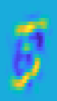
train_tilde_k = F*Vk';

Below is a reprojection of a training image which was represented in eigenspace with k eigenvectors. It can be observed as the explained variance approaches 1, the reprojection approaches the original image.

sample = 1;
figure(2)
subplot(1,2,1)
imagesc(reshape(train_tilde(sample,:),[28,28]));
axis on
title("Original image sample")
subplot(1,2,2)
imagesc(reshape(train_tilde_k(sample,:),[28,28]));
axis off
title(sprintf("Reconstruction using %i eigenvectors",k))

The reduced matrix, eigenbasis, training labels and mean is saved to be used for classification.

save('trainPCA.mat','trainLabels','F','Vk','trainMean')

Prepare Test Data

The test data is prepared in a similar fashion to the training data. Due to the large set of test images it's recommended to use a subset of images.

numTest =500;
test = double(reshape(imgDataTest, [784,10000]))';
test = test((1:numTest),:);
testLabels = double(string(labelsTest(1:numTest)));

Project Test Images onto Eigenbasis & Back

The eigenbasis can now be tested on images outside the original dataset. If a good representation of has been found then the same subest of k eigenvectors should be able to recreate the new images.

Projection is again performed by .

test_tilde = test-trainMean;
test_k = test_tilde*Vk;

and reverse projection .

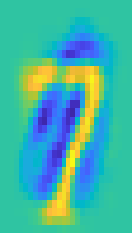
test_tilde_k = test_k*Vk';

As can be seen, below the recreation is not as accurate on the test set as the training set. This is expected as the basis has not been specifically calculated for the test set. However, as all images of digits are theoretically in the same domain, the representaiton is still able to convey most of the information from original image.

sample = 1;
figure(3)
subplot(1,2,1)
imagesc(reshape(test_tilde(sample,:),[28,28]));
axis on
title("Original image sample")
subplot(1,2,2)
imagesc(reshape(test_tilde_k(sample,:),[28,28]));
axis off
title(sprintf("Reconstruction using %i eigenvectors",k))

Classification of Image

Now that the orginal dataset has been projected onto the new basis, the class of novel images can be infered using the dataset labels. The overall approach to clasiffication is testing the distance between the transformed novel image and the known set of images in reduced dimensionality. In practice this can take many different forms however euclidian distance and k nearest neighbour were explored in this implementation. See the appendix linked from the title to see an explanation of each method.

Classification Scheme A - Euclidian Distance

The first classifcation scheme implemented is euclidian distance which, unfortunately proved to have low accuracy when evaluated on the test set.

correct = 0;
for i = 1:numTest
    [prediction, confidence] = euclidianDistance(trainLabels,F,test_k(i,:));
    if prediction == testLabels(i)
        correct = correct + 1;
    end
end

euclidian_distance_accuracy = correct/numTest

euclidian_distance_accuracy = 
   0.6580

Classification Scheme B - K Nearest Neighbours

A K nearest neighbours scheme was implemented and found to provide much higher classification accuracy than euclidian distance. K = 5 was found to provide the best accuracy with all other values default.

correct = 0;
for i = 1:numTest
    prediction = kNearestNeighbours(trainLabels,F,test_k(i,:),5);
    if prediction == testLabels(i)
        correct = correct + 1;
    end
end

euclidian_distance_accuracy = correct/numTest

k_nearest_neighbours_accuracy = 
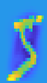
   0.8560

Below is an example of the standalone image classification function. This function uses K nearest neighbours, with K = 5 to classify the digit.

image = reshape(test(2,:),[28,28]);
classifyImage(image);

Conclusion

Reasonable compression and classification can be achieved using principal component analysis methods. By reforming the basis of the pixel space in terms of the most relevant 'principal' components, the images can be recreated in a much smaller dimensionality while still preserving the information. With the inital settings; a dataset of 1000 images, and an explained variance of 0.7, the images can be represented with only 3% of the original information.

Specifically with MNIST and other image processing tasks, PCA exhibits weaker performance than machine learning techniques such as convolutional neural networks. As the original images are reshaped into a single vector, PCA doesn't respect the spatial relationships between pixels unlike CNNs. This issue becomes more obvious on datasets which are not pre-centered as PCA lacks invariance to translation.

PCA does however, beat out even simple machine learning solutions in terms of training and interpretation time.

Appendix A - Function prepareData

function [imgDataTrain, labelsTrain, imgDataTest, labelsTest] = prepareData
% Copyright 2018 The MathWorks, Inc.
%% Check for the existence of the MNIST files and download them if necessary

filePrefix = 'data';
files = [   "train-images-idx3-ubyte",...
            "train-labels-idx1-ubyte",...
            "t10k-images-idx3-ubyte",...
            "t10k-labels-idx1-ubyte"  ];

% boolean for testing if the files exist
% basically, check for existence of "data" directory
download = exist(fullfile(pwd, 'data'), 'dir') ~= 7;

if download
    disp('Downloading files...')
    mkdir data
    webPrefix = "http://yann.lecun.com/exdb/mnist/";
    webSuffix = ".gz";

    filenames = files + webSuffix;
    for ii = 1:numel(files)
        websave(fullfile('data', filenames{ii}),...
            char(webPrefix + filenames(ii)));
    end
    disp('Download complete.')
    
    % unzip the files
    cd data
    gunzip *.gz
    
    % return to main directory
    cd ..
end

%% Extract the MNIST images into arrays

disp('Preparing MNIST data...');

% Read headers for training set image file
fid = fopen(fullfile(filePrefix, char(files{1})), 'r', 'b');
magicNum = fread(fid, 1, 'uint32');
numImgs  = fread(fid, 1, 'uint32');
numRows  = fread(fid, 1, 'uint32');
numCols  = fread(fid, 1, 'uint32');

% Read the data part 
rawImgDataTrain = uint8(fread(fid, numImgs * numRows * numCols, 'uint8'));
fclose(fid);

% Reshape the data part into a 4D array
rawImgDataTrain = reshape(rawImgDataTrain, [numRows, numCols, numImgs]);
rawImgDataTrain = permute(rawImgDataTrain, [2,1,3]);
imgDataTrain(:,:,1,:) = uint8(rawImgDataTrain(:,:,:));

% Read headers for training set label file
fid = fopen(fullfile(filePrefix, char(files{2})), 'r', 'b');
magicNum  = fread(fid, 1, 'uint32');
numLabels = fread(fid, 1, 'uint32');

% Read the data for the labels
labelsTrain = fread(fid, numLabels, 'uint8');
fclose(fid);

% Process the labels
labelsTrain = categorical(labelsTrain);

% Read headers for test set image file
fid = fopen(fullfile(filePrefix, char(files{3})), 'r', 'b');
magicNum = fread(fid, 1, 'uint32');
numImgs  = fread(fid, 1, 'uint32');
numRows  = fread(fid, 1, 'uint32');
numCols  = fread(fid, 1, 'uint32');

% Read the data part 
rawImgDataTest = uint8(fread(fid, numImgs * numRows * numCols, 'uint8'));
fclose(fid);

% Reprocess the data part into a 4D array
rawImgDataTest = reshape(rawImgDataTest, [numRows, numCols, numImgs]);
rawImgDataTest = permute(rawImgDataTest, [2,1,3]);
imgDataTest = uint8(zeros(numRows, numCols, 1, numImgs));
imgDataTest(:,:,1,:) = uint8(rawImgDataTest(:,:,:));

% Read headers for test set label file
fid = fopen(fullfile(filePrefix, char(files{4})), 'r', 'b');
magicNum  = fread(fid, 1, 'uint32');
numLabels = fread(fid, 1, 'uint32');

% Read the data for the labels
labelsTest = fread(fid, numLabels, 'uint8');
fclose(fid);

% Process the labels
labelsTest = categorical(labelsTest);

disp('MNIST data preparation complete.');

end

                    

function [prediction, confidence] = euclidianDistance(labels, F, test)
n = size(F);
distance = zeros(1,10);
count = zeros(1,10);

for i=1:n(1)
    ind = labels(i)+1;
    distance(ind) = distance(ind) + sqrt(sum((F(i,:)-test).^2));
    count(ind) = count(ind) + 1;
end

for i=1:10
    distance(i) = distance(i)/count(i);
end

distance = sum(distance)-distance;
confidence = distance/sum(distance);

[~, prediction] = max(confidence);
prediction = prediction - 1;
end
                    

function prediction = kNearestNeighbours(labels, F, test, K)

n = size(F);
distance = zeros(n(1),1);

for i=1:n(1)
    distance(i) = sqrt(sum((F(i,:)-test).^2));
end

[~, I] = sort(distance);
temp = zeros(K,1);
for i=1:K
    temp(i) = labels(I(i));
end

prediction = median(temp);

end
                    

function prediction = classifyImage(image)
if (~exist('trainLabels','var') || ~exist('F','var') || ~exist('Vk','var') || ~exist('trainMean','var'))
    try
        load('trainPCA.mat')
    catch exception
        disp('Required variables not found, please run training section')
        throw(exception)
    end
end

image = double(reshape(image,[784,1]))';

X_tilde = image-trainMean;
X_k = X_tilde*Vk;

prediction = kNearestNeighbours(trainLabels,F,X_k,5);
figure(4)
imagesc(reshape(image,[28,28]));
axis off
title(sprintf('Digit is predicited as %i',prediction));
    
end